More Gocad

This will give you another worklfow for using Gocad to model a faulted surface. The workflow we do here is a little different from the other faulted Gocad primer; both are valid workflows. This tutorial needs Gocad 2009.1 or higher.

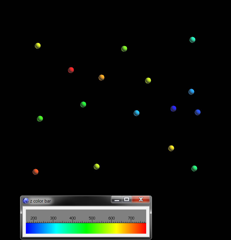
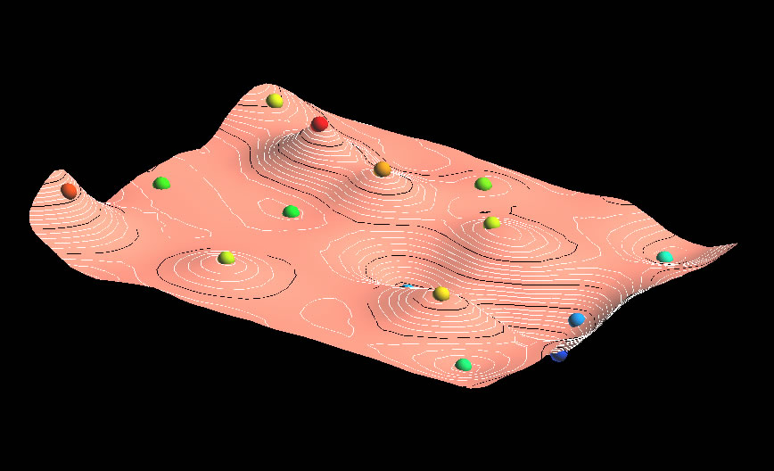
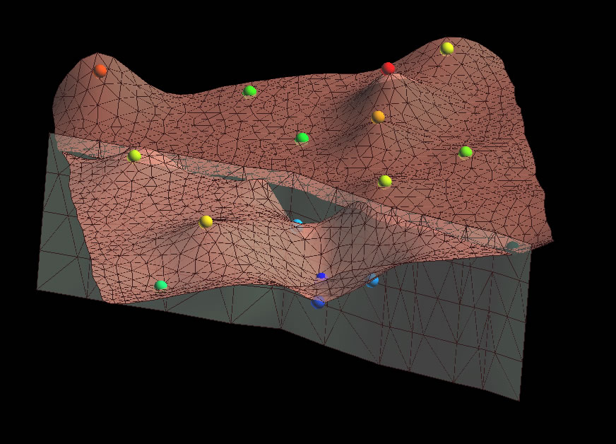
Our dataset is the points you hand contoured earlier in class. I have loaded these into a Gocad project called handCont.gprg on Q:\Courses\Geo 335-Petroleum\Gocad_primers. Recall that there is a high in the NW and a low in the east (Warm colors are high, cool colors are low).

Just as with hand contouring there are many ways to honor the same data, and to incoporate other ideas, such as the structural style in an area. For example what if we thought this were data of bed that were extended by faulting?  How could we incorporate normal faults?  Traditionally one would contour by hand each fault block separately bound by a line that represented the fault through that bed.  We will sort of do this, but in 3-D with the fault as an actual surface. 

Our approach will be to create a fault and then cut an uninterpolated surface with the fault and then interpolate each surface (fault block) separately.  In order to make the fault we will draw the trace of the fault on a surface then move this trace, in effect making contours of the fault.  If you choose to do it this way, you should be mindful that any dip you are making is implicit the spacing of contour lines. You should use trig to determine this accurately (draw a sketch to figure it out).

Here are the steps:

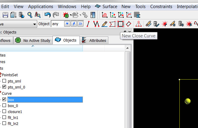
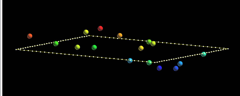
1. Make a box around the data.

2. Densify the box to something meaningful, in this case 1000 ft., using the Curves-> Tools-> Densify menu.

Note that the default elevation of the curve is the average of any visable object (in this case the points).

3. Build a surface using the menu Surface-> New-> From Closed Curve.

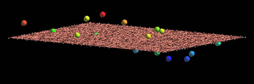
If you wanted to make a surface WITHOUT FAULTS, it would be easy, you would just set the constraints and run the interpolation, as you did with the previous tutorial and you would be honoring the data.

4. But we want to consider the possibility of normal faults. The most logical place is to put a graben where the low (blue) points are.

We do this by first cutting the surface, then interpolating.

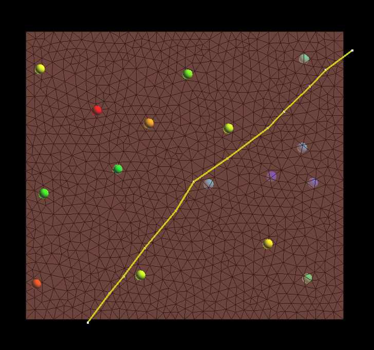
5. Take the surface you made from the box and draw a line or two where you think the fault traces on the surface should be.

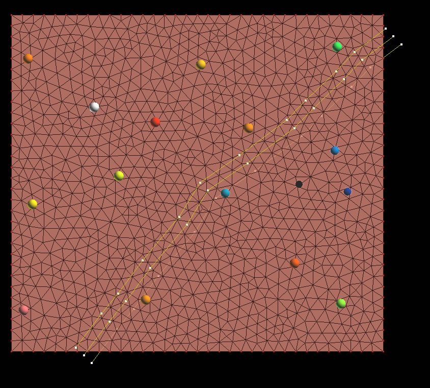
6. Then copy the line twice and translate it with Curve-> Tools-> Part-> Translate. The amount you translate it will depend on what you want these to fault contours to represent in the real world. That is Vc= sqr(x^2 + y^2) and Hc = z, where Vc and Hc are the vetical horizontal components of the fault in the dip direction.

You can and must use trig to figure out what you want these values to be for your own projects, such as 60 deg for normal faults, or other constraints you have, such as fault cuts between wells. Just translating the fault contour willy nilly is not acceptable. For this case use x = -700, y =700 and z =1700 for translation of the one fault contour line. This is a vector, so for the other fault contour line use negative of this vector.

7. Make a fault from the menu Surface-> New-> Several Curves. Then cut the horizon surface with the fault surface: Surface-> Tools-> Cut by Surfaces.

Great, except that we if we interpolate at this point (after setting the constraints, like primer #1), we will not get a very satisfying faulted surface. Notice how the throw is jumping all over as you move along the strike of the fault. This is because the initial elevation of the surface was based on the average of the points. The interpolation modifying from an initial starting point.

8. So, what we really want to do is have the horizons on either side of the fault honor the data at the fault, and show a generally consistent offset. One way to do this is by making each surface have their own starting elevation across the fault.

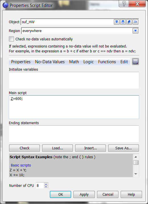
Make a couple of copies of your original, uninterpolated surface. Then offset them some nominal value. Assign the Z value of the footwall to be 200 ft by choosing the menu Compute>On Object and then completing the dialog box as follows (NOTE YOU MUST FOLLOW AN EXPRESSION WITH A “;” to end the expression. Do the same for the haningwall, assigning it to be 600.

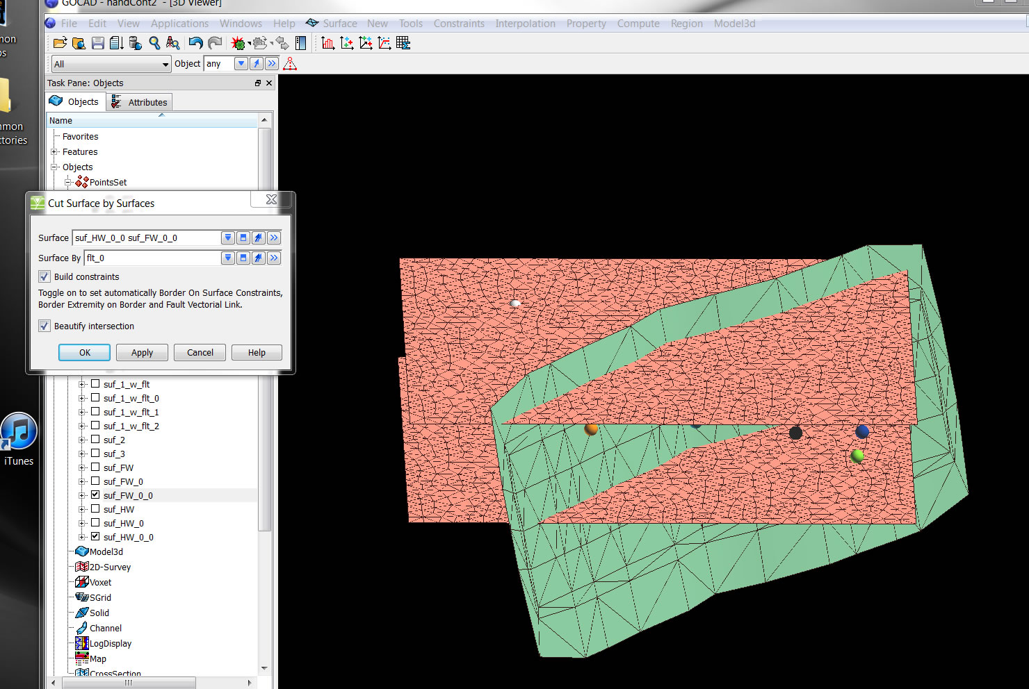
9. Cut the HW and FW by the fault.

10. Then delete the blocks you don't need with Surfaces-< Tools-> Part-> Delete Selection.

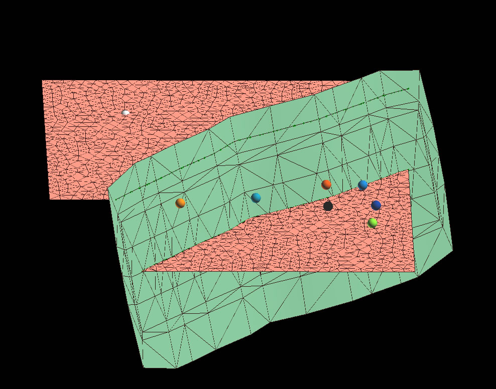
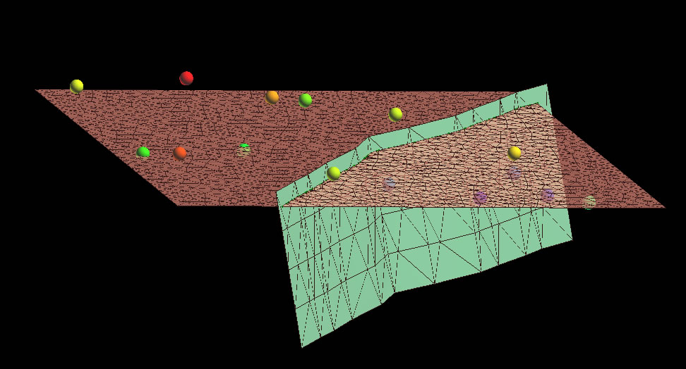
11. Now set constraints and run interpolation on each surface.

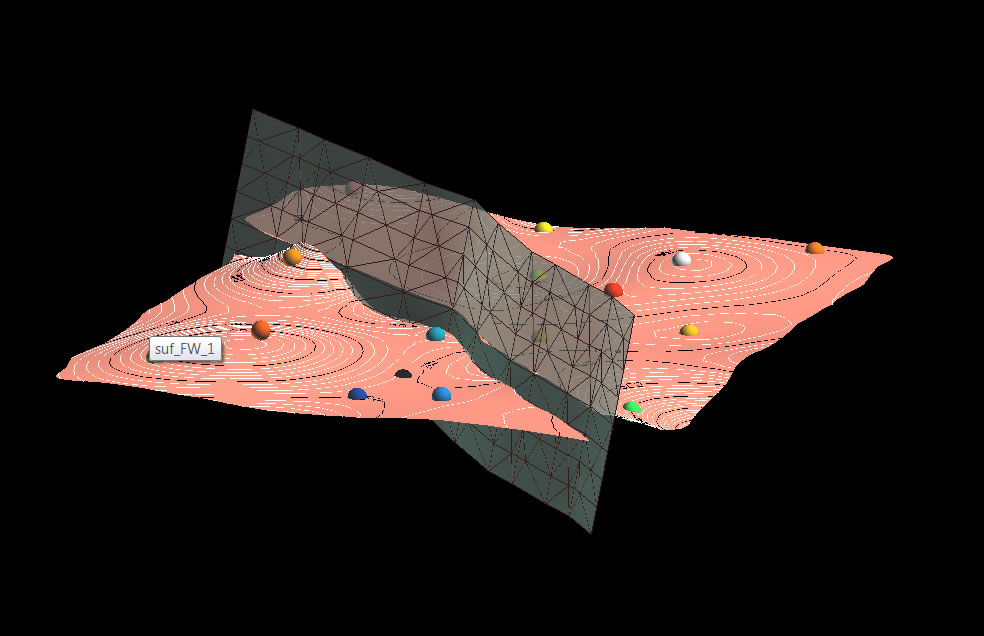
A few words about this. The surfaces are now much more reasonable, and the offset across the fault better than shown above in step 7. But they could still be improved. In this case the densification of the original box (and therefore the number of triangles generated) was probably too high. Furthermore, more faults, or a different fault position, could have been put in as the orange point in the left side more reasonably belongs on the FW. Finally, psuedo points could have been added (which could act as more constraints) would make the fit on the upper left better.

Connors, '12