Surfaces and Grids in Matlab

The ability to handle surfaces and grids is one of Matlab’s many strengths.  Since a lot of geologic data is naturally of more than one dimension, we have use for these capabilities. 

Surfaces

A surface is a set of polygons.  They are easy to plot in Matlab. Because data is often not regularly sampled, surfaces are often modeled as a set of interlocking triangles.  There is a particularly compact way of making surfaces of irregularly spaced data called a Delaunay triangulation.  Delaunay triangulation is the set of triangles built by connecting each of the points of an irregularly spaced data set where the vertices of the triangles are the data points.  Thus it is an exact representation of your known data and linear interpolation in between. 

To see what we mean, load up the dmap.dat data file from the Q:\geo185 directory by typing “load dmap.dat”

This is an X,Y,Z elevation data file for columns 1,2,3.

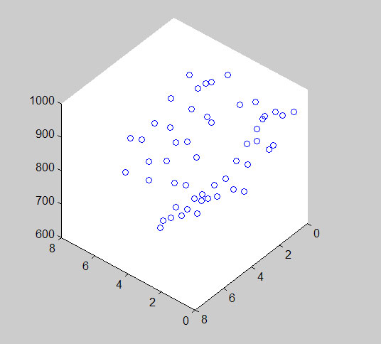
First visualize the file with the “plot3” command

>> p_h=plot3(dmap(:,1),dmap(:,2),dmap(:,3),'o')

The 'o' parameter plots the data points as individual circles as opposed to a 3D-line.

The “p_h” is called a handle.  You could have just typed plot3… without the “p_h” but by adding this you have the ability to later delete this graphic element

>> hold on

This keeps the plot held for more plotting

Now in order to plot the data as a triangulated surface we need to build the surface first with:

>>tri=delaunay(dmap(:,1),dmap(:,2))

This creates a n x 3 matrix of the vertice row entries that are needed for each triangle

to visualize this triangulated surface type:

>> trisurf(tri,dmap(:,1),dmap(:,2),dmap(:,3))

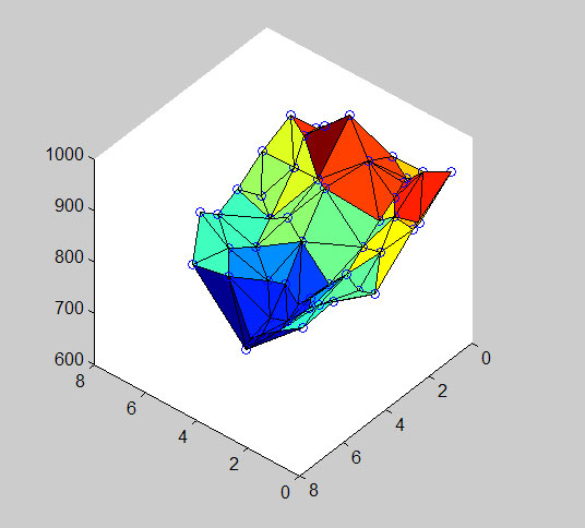
Note that the vertex of each triangle is one of the data points.

If you want to see the plot without the points type:

>>delete(p_h)

This surface plot is efficient but it doesn’t produce a very pretty picture (well at least for this small data set, for large data sets, triangulated surfaces are often preferable because they are more compact and there is enough data that the surface looks good).

Grids

So we often want a regular spacing of the X and Y locations to make it smoother and not faceted.  A regularly spaced data set is called a grid.  It uses up more memory and thus is slower to manipulate because data is defined at every location.  To convert the irregularly spaced data to regularly spaced we need to grid it.  This requires a couple of steps.  First you need to define the spacing and extent of the grid by making two vectors of the X and Y upper and lower limits at a given spacing:

>> rangeY=floor(min(dmap(:,2))):.2:ceil(max(dmap(:,2)))

>>rangeX=floor(min(dmap(:,1))):.2:ceil(max(dmap(:,1)))

0.2 is the spacing I have chosen.  I was a little obscure in choosing the “floor(min…” syntax.  Try “min(dmap(:,2))” to see what that gives you and then try “floor(min(dmap(:,2)))” to see what that does.  Hint: it is a way of controlling the rounding direction.

Now make matrices for each X and Y location:

>>[X,Y]=meshgrid(rangeX,rangeY)

And then interpolate your Z values across this grid:

>>Z=griddata(dmap(:,1),dmap(:,2),dmap(:,3),X,Y)

To see the result:

>>surf(X,Y,Z)

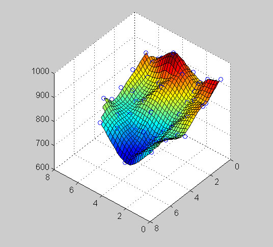
For a smoother interpolation add the “cubic” spline parameter:

>>Z=griddata(dmap(:,1),dmap(:,2),dmap(:,3),X,Y,'cubic')

>>surf(X,Y,Z)

Note that the grid values in between the data points vary smoothly and no longer have the facets we saw with the triangulated surface.

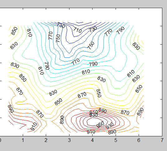
If you want to make a contour plot of the gridded data you can do this by first defining the range and spacing of the Z values:

>>rangeZ=floor(min(dmap(:,3))):10:ceil(max(dmap(:,3)))

Then running:

>>[C,h]=contour(X,Y,Z,rangeZ)

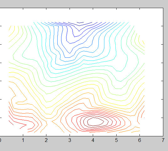
This makes a 2-D contour plot.  Again you could left off the “[C,h]” as this is a handle, but it is useful for labeling the contour lines:

>>c_h=clabel(C,h,rangeZ(1:2:end))

I chose to take every other value within “rangeZ”

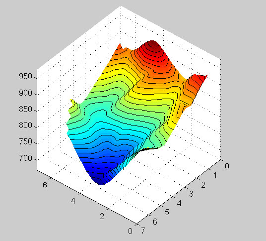
You can actually combine contours and surfaces and make your surface plot look better and with no grid lines:

>>surf(X,Y,Z,'EdgeColor','none','FaceColor','interp','FaceLighting','phong')

And then add 3-D contour lines:

>> contour3(X,Y,Z,rangeZ,'k')

There are many more possible plots with surfaces and grids.  I strongly urge you to look at the help files.

C. Connors, 2004, updated 2010